Bid shading. Bid landscape forecasting (Part 2)

November 2023

How can we approximate the win probability function?

Introduction

As demonstrated in the previous article, the optimal bid is determined by solving the following optimization problem:

\[b^*=\argmax_{b} (\hat{v}_x - b) w(b, x)\]

To determine the optimal bid for an auction, we require knowledge of the market price distribution, specifically the Cumulative Distribution Function (CDF) \(w(b)\).

By logging auction events where wins and losses occur, we can establish this dependency while addressing a binary classification problem. However, this process presents several challenges, such as selecting the appropriate class of functions and defining the loss function.

Bid landscape approximation

Let’s consider the pros and cons of choosing logistic regression and gradient boosting as predictors.

Logistic regression

In [1], the following formula is proposed:

\[w(b, x) = \frac{b^\alpha}{b^\alpha + c}\]

It is easy to demonstrate that this is equivalent to logistic regression: \(w(b, x) = \sigma (\alpha \log(b) - \log(c))\) where \(\alpha\) is a non-trainable parameter. As a generalization, we can consider: \(w(b, x) = \sigma (w_0 \log(b) + \langle w, x \rangle)\), which is essentially logistic regression.

Pros:

A. In [1], for particular cases (\(\alpha=1, \alpha=2\)), we can derive a closed-form formula for \(b^*\), eliminating the need to solve an optimization task during bidding.

B. utility function is convex

Cons:

A. If the market price does not follow a unimodal distribution, the function may fit poorly and could result in inefficiencies in bid shading

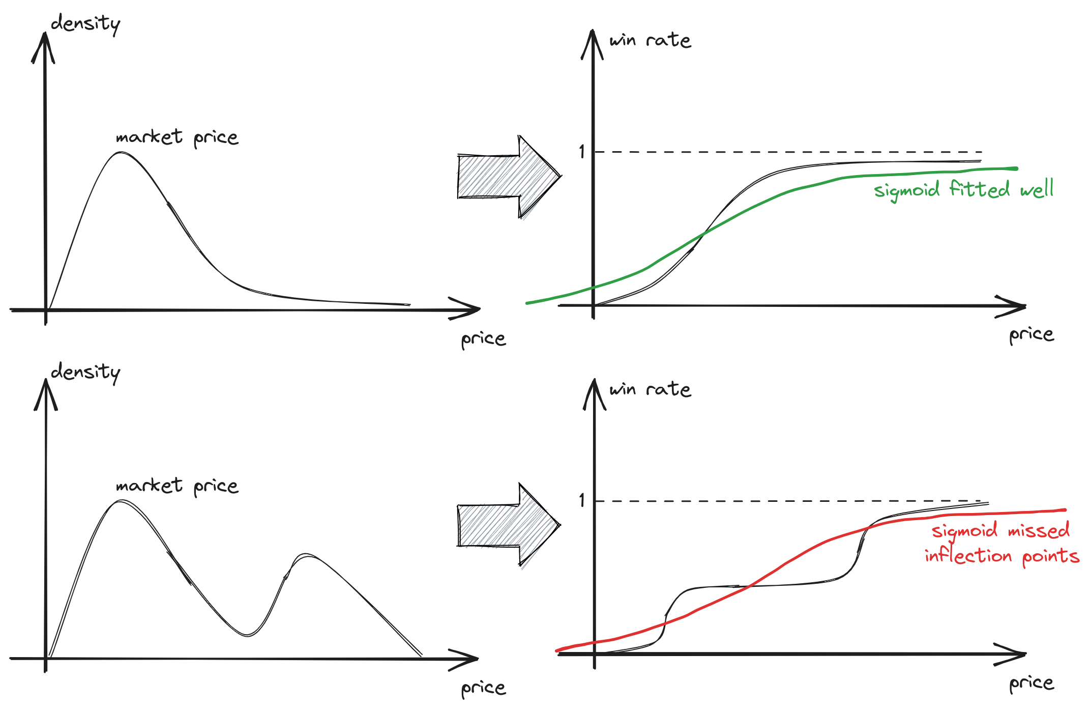
fig 1. Multimodal market price distribution poorly fitted by logistic regression

As shown in previous article, as the market price distribution becomes smoother, bid shading tends to be less efficient

B. The same slope is shared for all ad segments

For sigmoid function \(w(b, x) = \sigma (w_0 \log(b) + \langle w,x\rangle)\), \(w_0\) is the slope and represents the “variance” of market price, \(\langle w,x\rangle\) represents the mode of market price distribution.

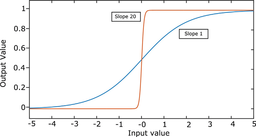
fig 2. different values of slope in sigmoid

If we aim to construct a generalized win probability predictor for various ad segments denoted as \(x\) and efficiently adjust bids for each segment, we need to fit a unique slope for each ad segment, i.e., \(w_0 = w_0(x)\). Such capability isn’t something that logistic regression can provide. Consequently, when dealing with multiple ad segments, we typically end up fitting an ‘average’ bell-shaped market distribution. However, this approach may not be suitable for scenarios where a specific segment exhibits a constant market price, and we want to apply effective bid discounts in such cases.

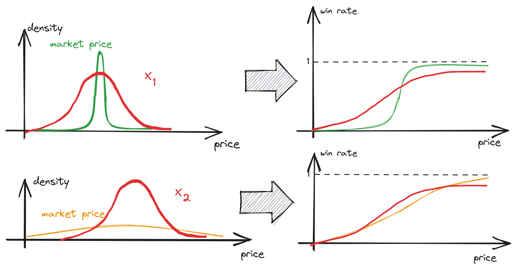
fig 2. All ad segments covered by the same “bell-shaped” function (red), but with different intercepts

Gradient boosting

As an enhanced alternative to describe the win probability, gradient boosting can be chosen. It possesses opposite properties when compared to logistic regression

Pros:

A. can handle multimodal market price distribution

B. for each ad segment, the algorithm can fit a separate step-based \(w(b\mid x)\) dependency

Cons:

A. the optimal bid can be found by solving an optimization problem for each auction during bidding

B. utility function is not convex (see example from the previous article)

Other approaches

There are a lot of other approaches for bid landscape forecasting:

direct evaluating market price. The drawback of this approach is that it provides an estimate of the market price expectation; however, it does not yield the winning probability as a function of the bid price, which is necessary for finding the optimal bid (that is trade-off between margin and win-rate)
DNN models [2]
estimating the market price distribution by applying survival analysis utilizing observed second prices (Paragraph 3.3.3 [3])
consider using a parametric distribution for market prices, such as a log-normal distribution. However, in practice, such approaches may perform poorly, as the real-world bidding landscapes are much more complex environments

Optimization

The main question is how we should optimize the model. One approach is to optimize the win probability model by maximizing likelihood. But does the task is to get accurate win probability estimates? We aim to find optimal bids for each auction. Let’s consider a toy example

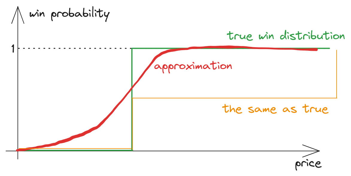
fig 3. More accurate win model produce worse bids

Let’s we know ideal win probability function \(w_{true}(b)\) (green). We approximated it by some model (red). Let’s consider another model (orange):

\[w_{synth} = \begin{cases} 0.5w_{true}(b), & \text{if } b < \infty \\ 1, & \text{b = } \infty \end{cases}\]

Clearly, in this case, the red line provides more accurate estimates of win probabilities, resulting in a much better log loss compared to the synthetic orange model. However, let’s consider the utility optimization problem: if we divide all win probabilities by two, the optimal bid remains the same! Therefore, the orange model yields more accurate optimal bids. In initial task, we are more concerned about the shape of the win probability function rather than its accuracy.

Let’s attempt to formulate the optimization task in a more precise manner. A perfect win function, denoted as \(w(b, x)\), produces perfect bids: \(b^* = \argmax_b (\hat{v}_x - b) w(b, x)\). We aim to find an approximation, denoted as \(\hat{w}(b, x)\), such that the resulting bids: \(\hat{b} = \argmax_b (\hat{v}_x - b) \hat{w}(b, x)\) are closer to the optimal ones. In other words:

\[\min_{\hat{w}} \Epsilon_x\lVert (\argmax_{b} (\hat{v}_x - b) w(b, x) - \argmax_{b} (\hat{v}_x - b) \hat{w}(b, x)) \rVert\]

By setting derivative of each term to zero, we get:

\[\frac{w'(b^*, x)}{w(b^*, x)} = \frac{1}{v-b^*} \\ \frac{\hat{w}'(\hat{b}, x)}{\hat{w}(\hat{b}, x)} = \frac{1}{v-\hat{b}}\]

\[\lVert \frac{w'(b^*, x)}{w(b^*, x)} - \frac{\hat{w}'(\hat{b}, x)}{\hat{w}(\hat{b}, x)} \rVert = \frac{\lVert\hat{b}-b^*\rVert}{(v-b^*)(v-\hat{b})}\]

So, to minimize error of optimal bid (\(\lVert\hat{b}-b^*\rVert\)), we should minimize the error of \(\frac{w'(b, x)}{w(b, x)}\). Let’s note that

\[\frac{w'(b, x)}{w(b, x)} = \frac{p(b, x)}{F(b, x)} = p(b, x | z < b)\]

where \(p(b,x)\) is PDF of market price, \(F(b, x)\) is CDF.This functional is analogous to the hazard function with covariates in survival analysis. Methods developed for accurately approximating such hazard functions could be applied to this task as well.

Takeaway

Approximating win probabilities with simple models can result in inaccurate estimations of optimal bids. More advanced models enable the forecasting of complex bid landscapes.
Fitting the right model can be challenging because the optimization goal is non-standard. Nevertheless, in practice, constructing an accurate win probability model by maximizing data likelihood remains a straightforward and highly efficient approach.