Bid shading. Intuition (Part 1)

November 2023

How does bid shading work, and what is the intuition behind it?

Introduction

Bid optimization is a critical component in modern bidders. Although it is known that simply bidding with impression value is the optimal strategy for 2-price auctions, it is essential to utilize market price information in 1-price auctions. Many companies have proven that bid shading can enhance the efficiency of buyers up to 20% [1].

This problem is well-formulated mathematically, and various strategies have been proposed. We consider one that is widely used: the maximization of total impression value subject to a budget constraint [2, 3]. In other words, we aim to minimize CPA while guaranteeing full budget utilization:

\[\max_{b_t} \sum_{t=1}^{T} v_t w_t(b_t) \\ \sum_{t=1}^{T} b_t w_t(b_t) = B\]

Here:

\(t\) - auction number, \(T\) - is the total amount of auctions for considered period, \(B\) - budget for considered period
\(v_t\) - impression value estimate for auction
\(b_t\) - bid price
\(w_t\) - win probability of the auction

By using method of Lagrange multipliers this optimization task can be rewritten:

\[\max_{b_t} \sum_{t=1}^{T} (v_t - \lambda b_t) w_t(b_t)\]

Let’s set \(\hat{v} = \frac{v}{\lambda}\) and optimize each \(b_t\) independently:

\[\max_{b} (\hat{v}_x - b) w(b, x)\]

We may think of \(\hat{v}\) as a \(\lambda\)-adjusted impression value. Intuitively, depending on the budget \(B\), impression values are scaled to guarantee budget delivery. Estimation of \(\lambda\) is beyond of scope of this article.

Next, we will discuss the intuition behind that formula and explore the properties of the resulting bids.

Intuition

\[\textcolor{green}{utility(b)} = \textcolor{red}{(\hat{v}_x - b)} \textcolor{blue}{w(b, x)}\]

The optimal bid is derived from maximizing a function composed of two components:

margin - Represents the money savings. It is a monotonically decreasing function.
win probability - Indicates the win rate. It is a monotonically increasing function.

If you bid low, your margin is high but your win rate is low, and vice versa. Thus, the optimal bid price for each particular auction is somewhere in the middle.

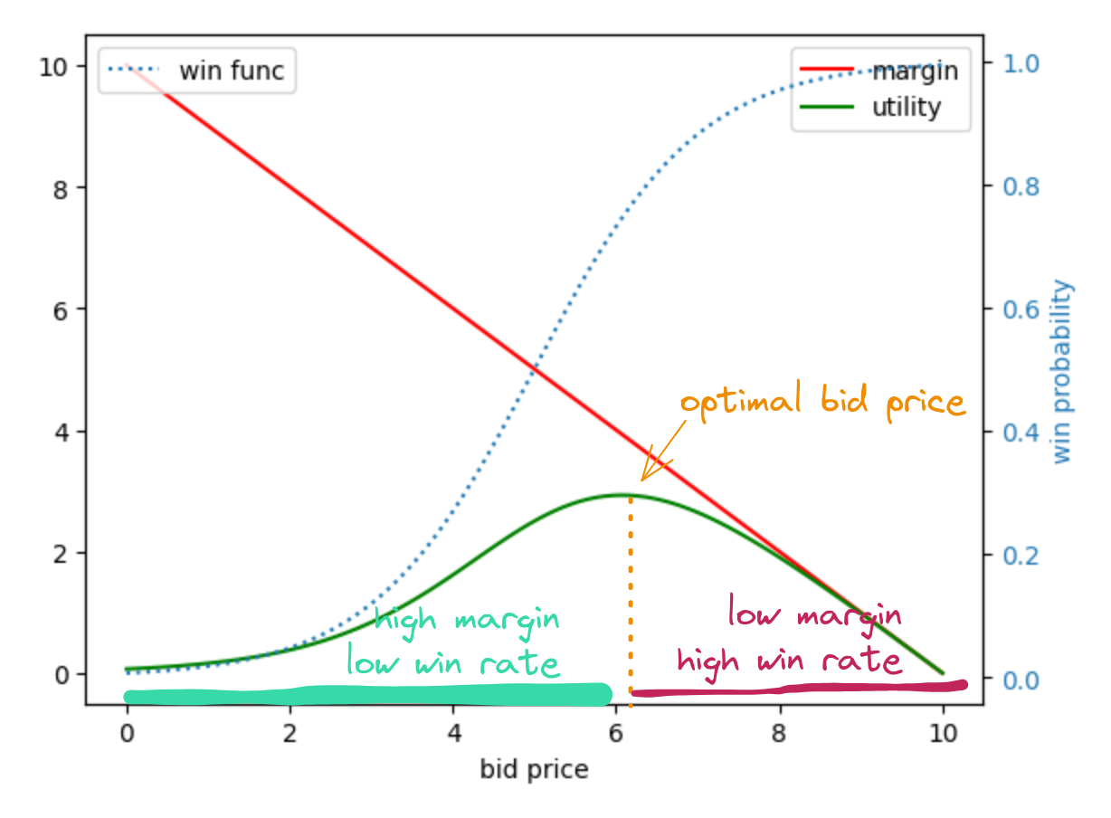
fig 1. The optimal bid is a trade-off between a higher margin and a reasonable win rate

Utility function is not convex in general

For example, if your win rate is modeled as a step-based function with high step values, the utility function would have a saw-toothed shape. Therefore, using general optimization methods (designed for convex tasks) would lead to achieving sub-optimal bids.

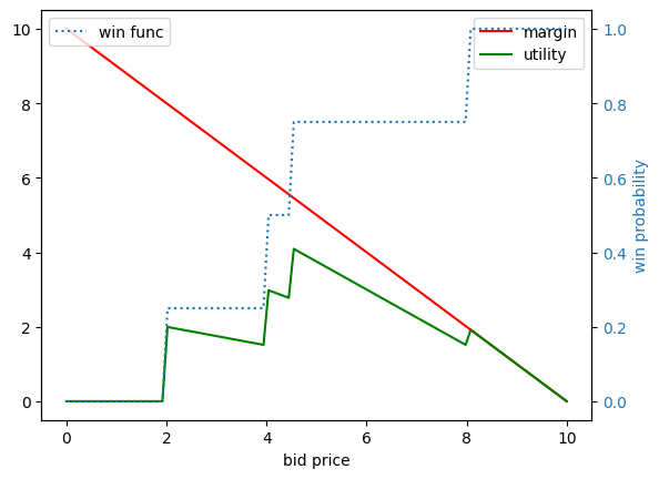
fig 2. Example of non-convex utility function

In which situations are bids discounted more?

What does a buyer want from a “bid shading” approach? If the impression valuation is significantly higher than the market price, they’d like to lower the bid to save money while still securing a win in the auction (without experiencing a significant decrease in the win rate). Conversely, if the impression valuation is close to or below the market price, the buyer doesn’t want to shade bids. Let’s demonstrate that the algorithm produces bids that align with these preferences.

As \(w(b) = P(z < b)\), where \(z\) denotes the market price, this represents the Cumulative Distribution Function (CDF) for the market price.

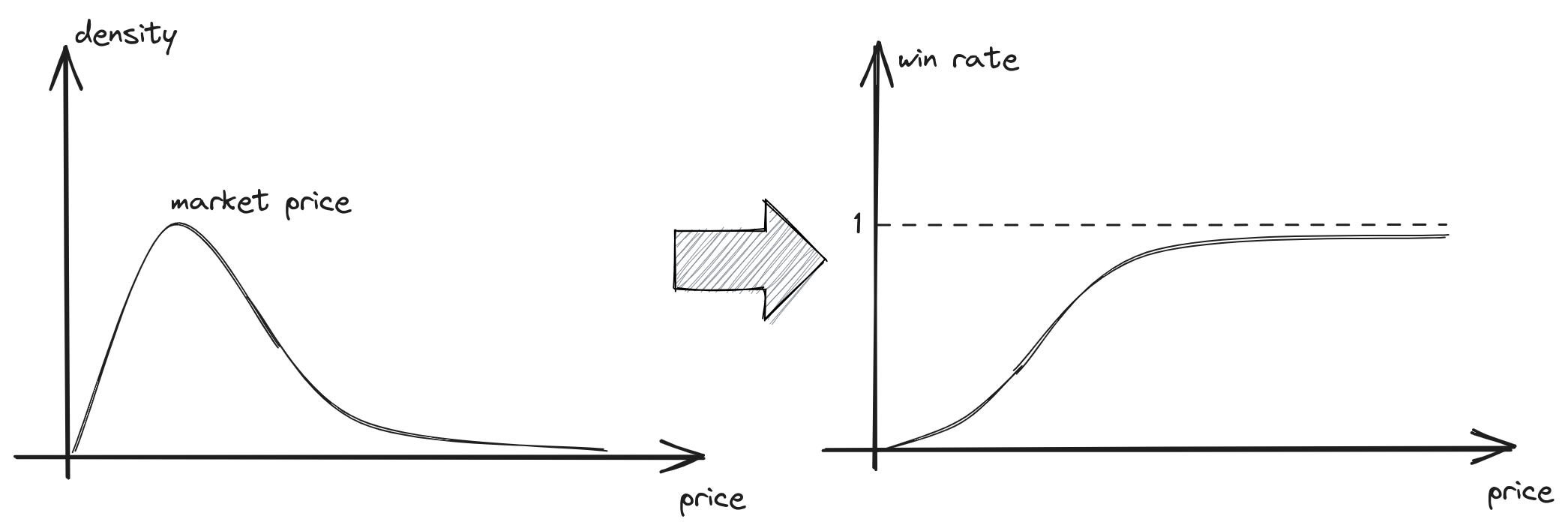
fig 3. Win rate is a cumulative distribution function of market price

Clearly, the optimal bid lies within the range \((0, \hat{v})\); otherwise, the utility would be negative. We can view bid optimization as the process of discounting the impression value. Analysing utility function for a specific value \(\hat{v}\), we might conclude:

When the valuation is in a range where the win-rate remains relatively stable, we could reduce the bid. This increases utility by expanding the margin without a significant decrease in win rate. Consequently, values will be discounted quite significantly. This situation commonly arises when:
1. \(\hat{v} \gg z\), leading to substantial savings.
2. \(\hat{v} \ll z\), the win rate here is typically low, making this case practically useless for consideration.
If valuation is proximate to the local mode of the market price distribution, any reduction in bid would also result in a notable decrease in win rate. Likely, we are in a region close to the local optimum of the utility function, and in this scenario, we shouldn’t anticipate significant value discounts.

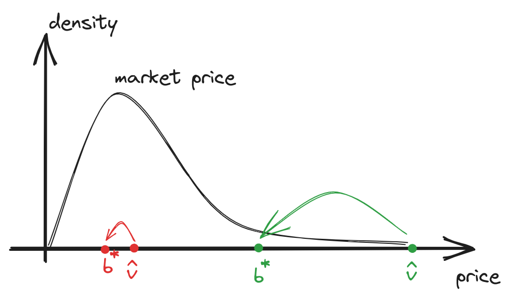
fig 4. Discounts depending on market price distribution and impression value

So the outcome of this strategy aligns well with the desired behavior: we aim to discount high-valued inventory closer to the market price, allowing us to save money.

How does the market landscape affect the efficiency of bid shading?

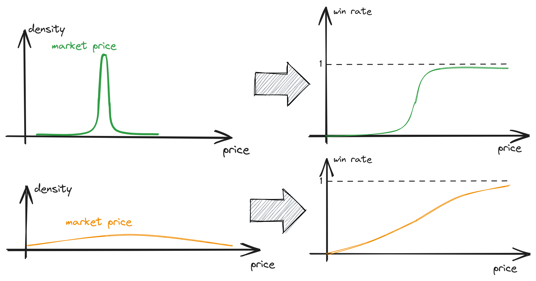
fig 5. Different market landscapes

The efficiency of bid shading varies based on the market price distribution:

If the market price is a delta-function, i.e., \(z = z_0\), then the optimal bid is consistently \(b^* = z_0\) (if \(\hat{v}>z_0\)). This is an ideal scenario where we don’t overpay.
For a market price with a uniform distribution, the optimal bid is always \(b^* = \hat{v}/2\). This is because the win rate remains constant and the utility function \(utility(b)\) is proportional to \((\hat{v}-b)b\). Given that \(\hat{v}\) represents the value divided by \(\lambda\) (which controls budget utilization), all values are discounted equivalently. As a result, this approach offers the same strategy as in 2-price auction: \(b = v\).

Where does the real profit lie?

On the one hand, we’ve outlined how bid shading helps us discount bids and save money. However, a counter-argument might be: “Yes, while my KPI improved, my spending decreased!”

Let’s refer to paragraph 3.2.3 [3]:

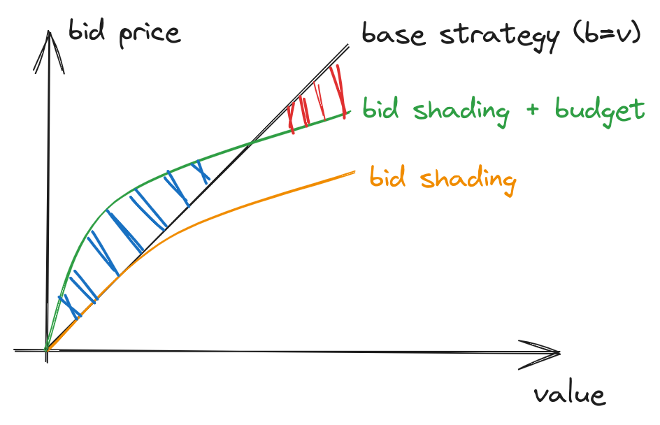
fig 6. Bid strategy expands spending for low-valued inventory

As discussed above, bids are discounted more for high-valued inventory. Therefore, the range between the orange and black curves represents the money saved by the algorithm. However, due to budget constraints and the need to match the spending of the base strategy, \(\lambda\) starts decreasing, and \(\hat{v}\) increases. As a result, the green curve representing the optimal strategy continues to save money on high-valued inventory (the red region) and reallocates these extra funds to low-valued inventory (the blue region).

In other words, the strategy accomplishes the following:

It saves money by discounting high-valued inventory closer to market price. (the red region)
It reallocates the saved funds to low-valued inventory by increasing their bids. (the blue region)

This way, we not only purchase most of the inventory from the base strategy but also acquire additional low-valued inventory. This also could help to explore a new unseen inventory that is not presented in the training dataset and therefore user response model undervalues it

Takeaway

Bid shading can significantly enhance buyer’s KPI.
Depending on the market landscape, bid shading may not always be efficient.
Bid shading enables an increase in the win rate for low-valued inventory.