Self-stealing of Attribution in Mobile Advertising

October 2023

What negative outcomes might arise from high-frequency bidding in environments with significant feedback delays?

Introduction

When initiating an advertising campaign, determining the optimal impression frequency strategy is a crucial step. The ideal frequency cap often depend on various campaign characteristics including the type of campaign, the creative format, the budget, the nature of the brand etc.

In certain domains, a decision to install (buy) a product might occur several hours or days after seeing the ad. Delays in attribution can also arise due to technical limitations; for instance, in mobile advertising, a user might download the promoted app during the game session, but the installation doesn’t register by SDK until the user opens the app for the first time [1].

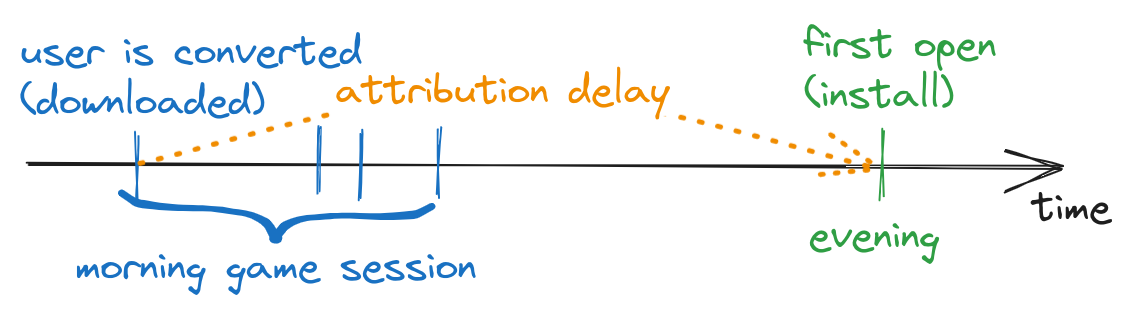fig 1. In mobile advertising, a high attribution delay could be caused by technical limitations

To address this, Mobile Measurement Partners (MMPs) use attribution windows [2]. Usually, a longer gap between the ad impression and attribution indicates a lower likelihood of user converted due to the ad impression.

This issue can create a sort of “attribution races” where the attribution is claimed by the ad network that interacted with the user most recently. For instance, imagine you displayed your ad to a user 5 times in a single day and then chose to stop showing the ad to avoid overexposure (since more impressions might discourage the user from making a purchase). But then, your competitor steps in and displays an 6th ad impression, which results in a sale. In this scenario, you essentially laid the groundwork for their success, potentially paying the price for their triumph.

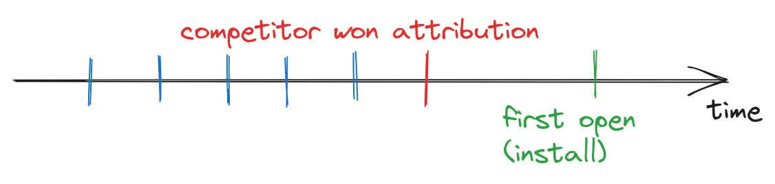fig 2. You showed an ad 5 times (blue), and user decided to convert. But competitor produced single impression in a right moment (red) and got the bank

Navigating attribution races can be quite challenging, as this is a game with information assymetry. But what about cases involving self-competition?

Self-stealing

Let’s refer back to the example from Figure 1. For a certain user, you receive 4 bid requests consecutively. What could potentially go wrong when you aim to evaluate the bid price for the 2nd, 3rd, and 4th bid requests?

If the user decides to convert after the first impression, we obviously shouldn’t bid thereafter. However, our confidence that the user didn’t convert increases as the lag from the first impression extends. By bidding after a short delay, the only outcome we might achieve is stealing the attribution from the first impression
Another challenge is if you want to build a model that predicts conversion (install), your train labels could be misassigned, and “1” would be assigned to the most recent (4th) impression. If you use such feature as “delay since the previous impression” - your model will “learn” to predict higher conversion probability straight after the previous impression and therefore bid frequency will increase. And the first impression in batch would be undervalued. Technically everything is correct: usually batch of two bids are more likely lead to attribution, but you spend twice. And due to selection bias your further trainset releases would be even stronger suffered from self-stealing.

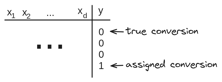fig 3. Conversion always assigned to the latest impression in the batch

Impression value discounting

Let’s consider two consecutive bid requests for a certain user at moments \(t_1\) and \(t_2\). We have also evaluated impression values \(v_1=v(x_1)\) and \(v_2=v(x_2)\). Here, by \(x\) we are considering all features and contextual information available at the bidding time.

A. For modeling delayed feedback the one common choice is exponential distribution [3]. So if impression occured at time \(t_0\), then conversion probability at time \(t\) is:

\[p(x, t) = p_0(x) e^{-\lambda(t-t_0)}/\lambda\]

As usually \(v(x) \sim p(x)\) we may use the following formula for value estimation:

\[v(x, \Delta t) = v_0(x)e^{-\lambda\Delta t}\]

One can interpret this formula as follows: once an impression is generated, it holds the highest value, but as time progresses and the likelihood of conversion diminishes, the remaining value approaches zero

B. Returning to our example. What is our dilema at time \(t_2\)? Actually we have two options:

not to bid: \(bid_2=0\), expected value of this action is \(v(x_1)e^{-\lambda(t_2-t_1)}\)
to bid: \(bid_2=b^*\), expected value of this action is \(v(x_2)\)

How to decide about \(b^*\)? The one approach is to maximize expected utility. But firstly, let note that “not to bid” is also have place even if \(bid_2>0\) but we didn’t win the auction. So if probability of win is a function \(w(b)\) then, our expected utility is:

\[\begin{aligned} E(utility(b^*)) &= v_1e^{-\lambda(t_2-t_1)}(1-w(b^*)) + (v_2 - b^*)w(b^*)\\ b^* &= \arg \max_{b^*}E(utility(b^*))\\ b^* &= \arg \max_{b^*}[(v_2 - v_1e^{-\lambda(t_2-t_1)}) - b^*]w(b^*) \end{aligned}\]

Let \(\hat{v}_2 = v_2 - v_1e^{-\lambda(t_2-t_1)}\). Then optimal bid is the solution of

\[\arg \max_{b^*}(\hat{v}_2 - b^*)w(b^*)\]

In other words, to take into account self-stealing we just need to adjust our impression valuation:

\[\hat{v}(x) = v(x) - v_{prev}e^{-\lambda \Delta t}\]

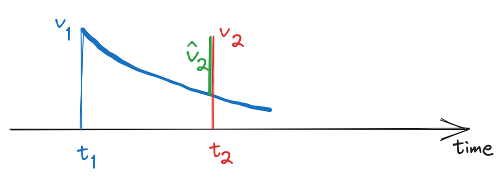fig 4. The larger \(t_2-t_1\) the smaller a discount

In a production system, implementing such adjustment could be quite straightforward. One would simply need to store the delay time from the previous impression, the value of that previous impression and also build a model that evaluates \(\lambda(x)\) for each particular bid request [3]

Budget constraint

At first glance, everything appears to be good: we have incorporated a simple discount term that can control the delay between impressions. However, the trade-off is that the algorithm is likely to spend less. Indeed, by discounting our valuations, we may encounter decreased bid prices and win rates, which would naturally result in reduced spending.

A real production system includes mechanisms for bid scaling to regulate budget allocation. Clearly, when we integrate a self-regulating discount factor, bid scaling will increase. Consequently, we can anticipate that the new strategy would yield higher bids when the delay from the previous impression is extended, and lower bids in response to frequent bid requests.

Experiment

To validate results let’s run some synthetic auction simulations. Although real production systems are very complex envoronments it is always useful to measure possible effects on vanila examples to “feel” the model.

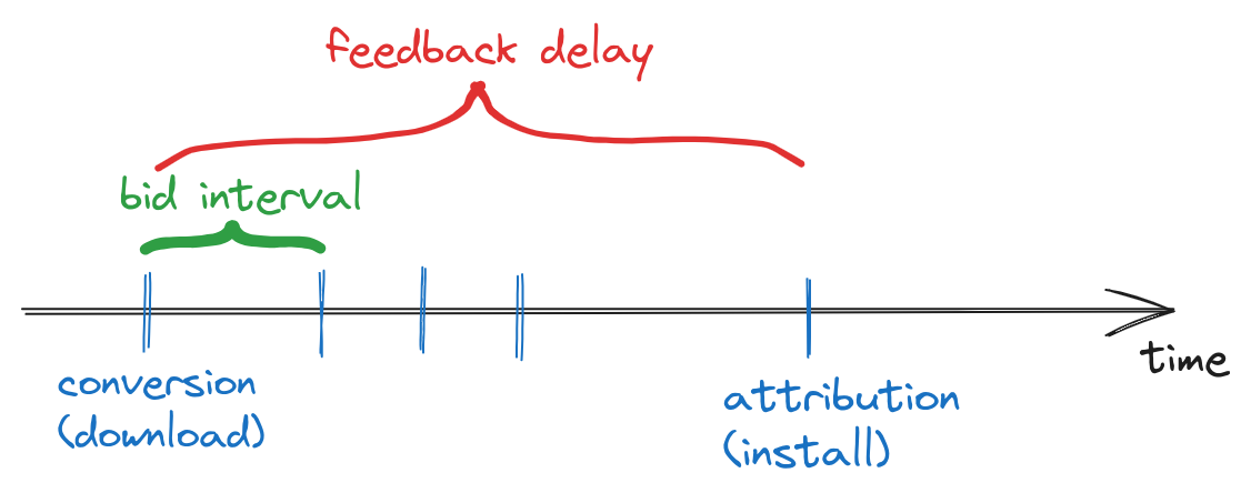fig 5. How feedback delay and bid intervals are related

The goal is to measure how some indicators are affected by ratio between average feedback delay and average bid interval.

if average feedback delay \(\texttt{>>}\) average bid interval – one can expect major effect from self-stealing.
if average feedback delay \(\texttt{<<}\) average bid interval – self-stealing is not expected to occur

fig 6. How bids are boosted depending on time ratio

The bid scaling ratio is a multiplier applied to the bids of the proposed strategy to maintain the same spending level as the default strategy. As mentioned above, discounting bids with small bid intervals can lead to significant drop in spend. So as expected, if feedback delays are huge - bids scaled signficantly comparing to baseline model (without discounting)

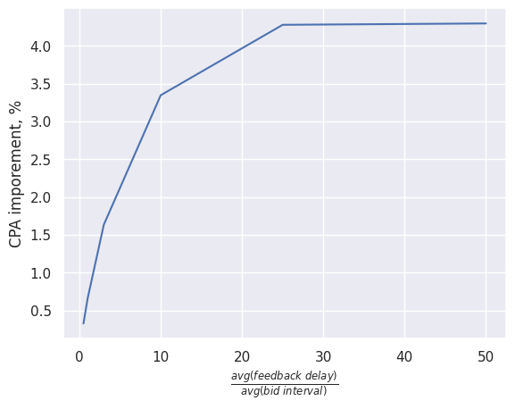
fig 7. How CPA are improved depending on time ratio

When the feedback delays are relatively high compared to the average interval between bids, those adjustments can yield percentages improvement in KPI.

Takeaway

Bidding environment with relatively high feedback delays or very low bidding interval (high frequency) present various challenges and increase the difficulty level of modelling. We considered the effects of ‘self-stealing’ and the negative consequences it can produce.
On one hand, messed train labels lead to reduced bid intervals, which amplify the effects of self-stealing. On the other hand, we considered a workaround (bid discounting) that pulls in an opposite direction - increasing bid intervals.
We conducted synthetic simulations to demonstrate that under certain conditions, the effects of ‘self-stealing’ would be significant.