How can we measure the impact of a new model, and what should we monitor?
Introduction
In a previous article, we demonstrated how introducing new features in bid landscape modeling can influence the performance. Another important step in enhancing your bidding strategy for performance advertising involves engineering new features into user response models. One can assume that adding informative features to the model would “improve the performance”. But what exactly should we monitor, and which KPI should show improvement? As usual, the answer varies; depending on the market landscape, you might see diverse or even contradictory results.
Let’s formalize our objective. In performance advertising, the private value of an impression can be assessed using the following formula:
\[value = p(A) * G\]
where \(value\) - impression value, \(p(A)\) - probability of conversion of event \(A\) and \(G\) - is a desired CPA of the campaign.
In the subsequent discussion, we’ll base our reasoning on a few assumptions:
- We assume that the user response model, \(p(A)\), is perfectly calibrated (which, practically speaking, is a very strong assumption): \(E(y) = p_a\). \(y=\{0,1\}\) and represents if conversion is occurred
- We don’t engage in bid shading; therefore, \(bid = value\).
While neither statement is true in practice, the subsequent analysis remains valuable. By examining ideal situations, we can gain a deeper understanding of complex systems like repeated auctions.
We aim to compare two models: the advanced model, \(p_a(x)\), which contains a newly engineered feature \(x\), and the base model, which does not include that feature: \(p_a = \Epsilon_x(p_a(x))\).
How is CPA affected?
\[CPA = \frac{\sum_i bid_i}{\sum_i I[y_i = 1]} = \frac{G \sum_i p_i}{\sum_i I[y_i = 1]}\]
Now, by substituting the denominator with the expected number of events and considering our assumption of the model’s perfect calibration, we obtain \(CPA = \frac{G \sum_i p_i}{\sum_i \Epsilon I[y_i = 1]} = \frac{G \sum_i p_i}{\sum_i p_i}\), which implies that \(CPA = G\). Thus, based on our bidding strategy’s design, the observed \(CPA\) always matches the desired one, regardless of the model’s complexity.
How has the spending changed?
The average spend can be determined by the expected spend in a single auction:
\[Spend = \Epsilon_x b(x) * F_z(b, x)\]
Where \(F_z(b, x)\) - win probability function (CDF of market price).
Expected spend of the base strategy:
\[Spend_{base} = b * F_z(b, x) = G*\Epsilon_x p_a(x) * F_z(G*\Epsilon_x p_a(x), x)\]
Expected spend of the advanced strategy:
\[Spend_{adv} = \Epsilon_x b_x * F_z(b_x, x) = G*\Epsilon_x p_a(x) * F_z(G*p_a(x), x)\]
Let’s conduct simulations to study the ratio \(R = \frac{Spend_{adv}}{Spend_{base}}\) within a log-normal market price distribution. A higher value of \(R\) indicates a greater impact of deploying the advanced strategy. To illustrate how the market landscape influences the efficiency of the advanced strategy, we’ll plot the dependency \(R(\mu)\), where \(\mu\) represents the average market price.
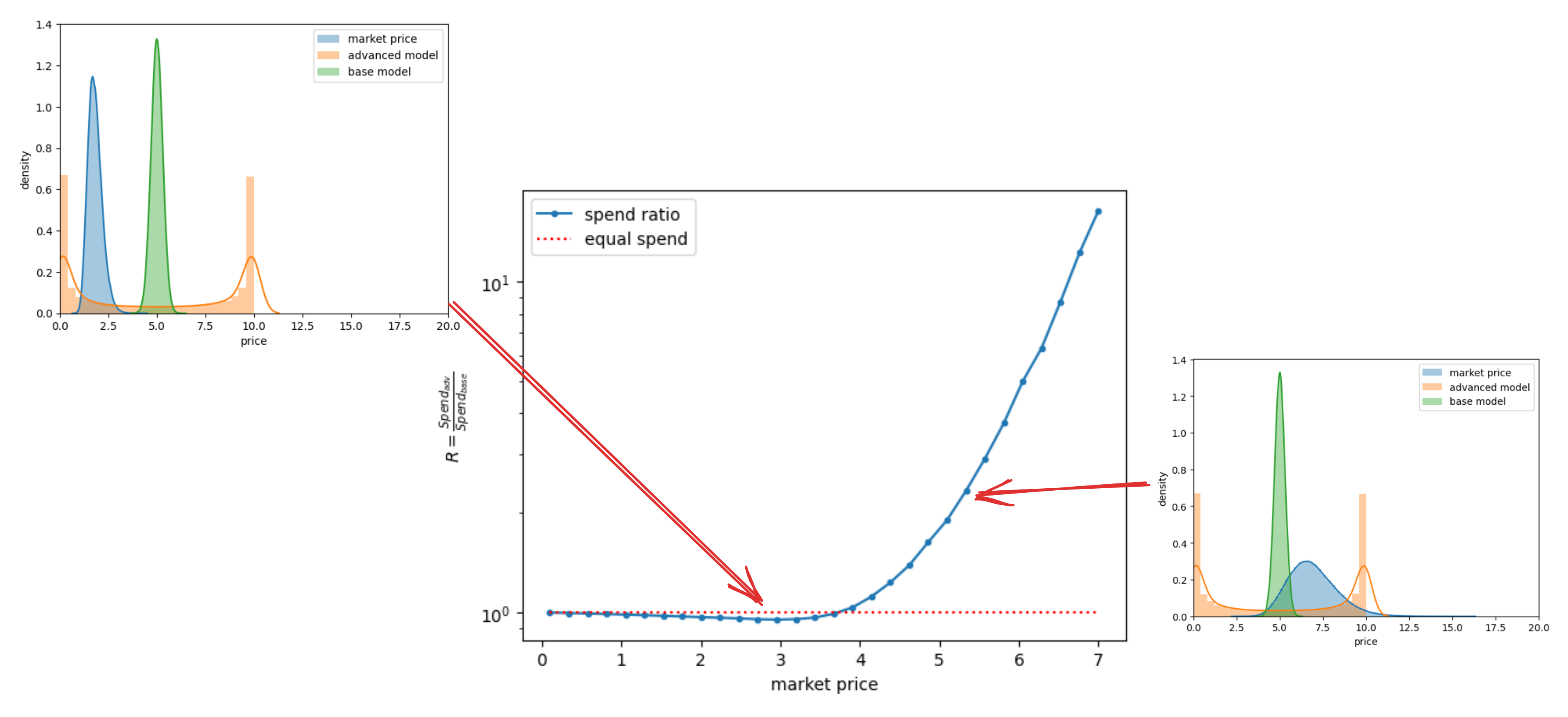
fig 1. How does the spending ratio correlate with the average market price?
Green: Bid price distribution of the base model.
Orange: Bid price distribution of the advanced model.
Blue: Market price distribution.
Why are the price distributions for Green and Orange so different? Let’s suppose we have a base model that is bell-shaped, as presented in the pictures. Now, we’ve introduced a superfeature that can separate high-conversion users. For such users, produced prices obviously become higher, so the Orange model has two peaks: the left peak for the average user and the right peak for prices for high-converting users.
We observe that in certain scenarios, the advanced model might spend less! This situation is depicted in the left image. When the market price is quite low, the base model might purchase all the available inventory, whereas the advanced model opts only for the high-valued inventory. However, as the market price increases, the impact of advanced features on spending becomes more pronounced, as seen in the right image.
High market prices typically indicate high competition. Therefore, it can be inferred that in competitive markets, robust new features significantly influence spending. Conversely, in markets with low competition and low prices, introducing new features may not offer any distinct advantages.
Example
To illustrate these effects, let’s delve into a straightforward example.
Imagine we have a single ad placement with a binary market price: $0.05 for half of the auctions and $0.5 for the other half (independently of user profile). This placement is represented by a total of 1,000 users. Now, suppose we’ve engineered a superfeature such that:
- 100 users have superfeature=1, and their conversion rate is 0.1.
- 900 users have superfeature=0, and their conversion rate is 0.01.
We’ll set a desired CPA of $10. If we disregard the superfeature, the average conversion rate is calculated as: \(\frac{100*0.1+900*0.01}{1000} = 0.019\).
Now, let’s examine the behavior of two models: the base one, which doesn’t account for the superfeature, and the advanced one that harnesses this information.
A. Base model
The base model will generate an identical bid for every user, calculated as:
\(b = 0.019 * 10 = \$0.19\). Since half of these bids exceed the market price, we will win 500 auctions. Then:
\[\begin{aligned}
Spend &= 500 * 0.19 = \$95 \\
Attributions &= 0.019 * 500 = 9.5 \\
CPA &= \$10
\end{aligned}\]
B. Advanced model
The advanced model will differentiate bids based on the superfeature. For users with superfeature=1, it will bid:
\(b = 0.1 * 10 = \$1\).
For users with superfeature=0, it will bid:
\(b = 0.01 * 10 = \$0.1\).
Clearly, we will win all auctions for users with superfeature=1. However, since half of the bids for superfeature=0 fall below the market price, we will not acquire those users.
\[\begin{aligned}
Spend &= 100 * 1 + 450 * 0.1 = \$145 \\
Attributions &= 0.1 * 100 + 0.01 * 450 = 14.5 \\
CPA &= \$10
\end{aligned}\]
From the analysis, it’s evident that both models yielded the same CPA, yet their spending behaviors differed. By tweaking the hyperparameters in this synthetic example, we could also produce opposite spending outcomes.
Takeway
- Feature engineering lets you spend more while hitting your target KPI. Real systems often have budget pacing. So, being able to spend more can lead to better KPIs without changing total spend (e.g. by lowering the target CPA).
- We talked about adding new features to the model. The same logic works when you make your model more complex - if you can better separate your audience, you may utilize more budget.
- When market prices are low, improving your model might not make a notable difference in performance.
- Making better models is tough, but setting up a live test the right way is even harder. If you track the wrong metrics, the test might fail and undo all your work, even if the new approach was better.