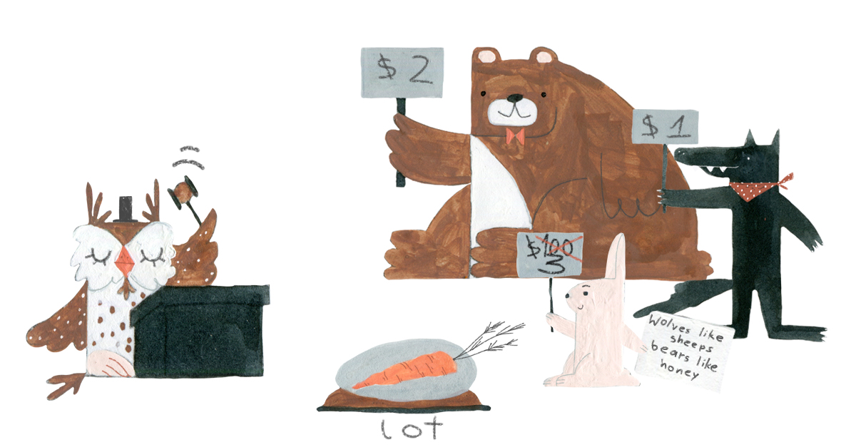
How can you avoid overpaying in auctions?
Introduction
Once the bid shading strategy is deployed into production, an interesting metric to monitor is how much we overpay for impressions. Fortunately, in many cases with winning bid callbacks, we have access to the second price. Thus, we can formulate the following metric:
\[E_x\frac{b_x}{E_z(z_x\mid z_x<b_x)}\]
where \(b_x\) - bid price, and \(z_x\) - is the second price (market price). This metric is evaluated over won auctions.
One could argue that if a bid strategy is designed perfectly, overpayment should be zero. However, due to the stochastic nature of the market price, there will always be some degree of overpayment. Moreover, this metric doesn’t accurately reflect how effectively we decide on bids; it merely represents the market landscape.
A common strategy is to estimate the expected value of the market price and place bids close to that value. Yet, if the variance of the market price is substantial, one can still end up overpaying significantly.
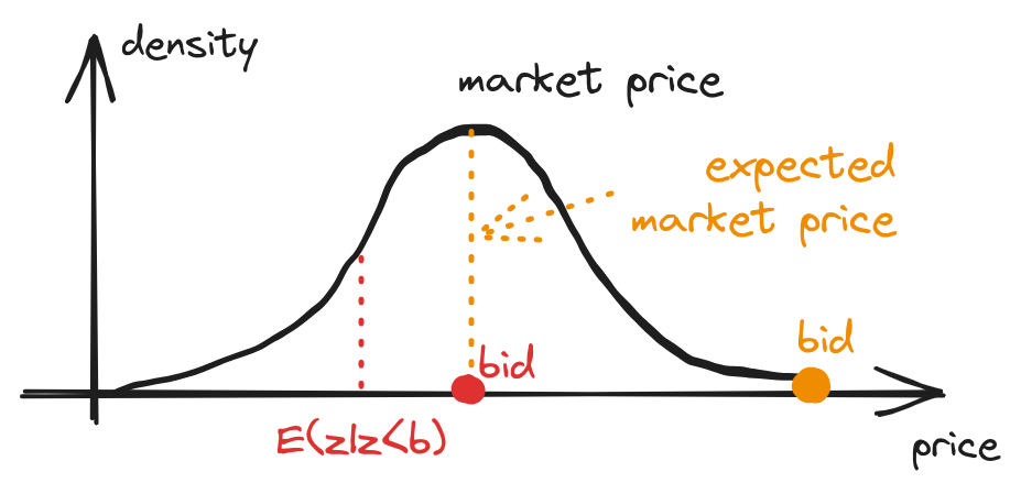
fig 1. Dashed vertical lines indicate observed market price for corresponding bid
The lowest overpayment ratio can be achieved in markets where the distribution of the market price is close to a delta function. In other words - in case of determenistic market price.
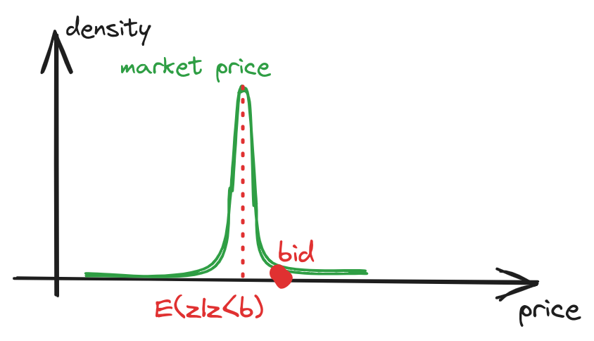
fig 2. The more determenistic market price - lower overpaying
Additionally, in theory, one can design a market price distribution in which the lower your bid, the higher your overpayment ratio:
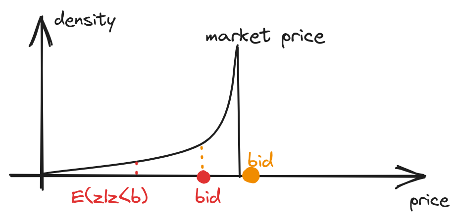
fig 3. Example of increasing overpay with lowering bid price
So, what can we conclude? Overpayment is a property of the market, and we can’t control it?
Reducing overpayments
Well, if we could somehow transform the market price distribution from a bell-shaped function to a delta-function, we could achieve lower overpayment.
It’s worth noting that we are analyzing the market price landscape for a specific ad segment, denoted as \(x\). What if we conditioned our market price model on a greater number of informative features? According to Law of total variance:
\[Var(z) \geq Var(E_x(z\mid x))\]
We can anticipate that as the market price variance decreases, overpayment will reduce.
Furthermore, with the reduction in variance, there is also an expected decrease in overbidding:
\[E_x\frac{b_x}{E(z \mid z<b, x) } \stackrel{?}{\leq} \frac{b^*}{E(z \mid z<b^*) }\]
Given that \(b_x\) is the solution to \(\argmax_{b}(\hat{v}_x - b) F_z(b, x)\), to prove that inequality analytically is indeed a challenging task.
Example. Log-normal market price distribution
Let’s examine this inequality in the case of a lognormal market price distribution
Let
\[\begin{aligned}
z &\sim LogNormal(\mu_0 + x, \sigma_z^2) \\
x &\sim N(0, \sigma_x^2)
\end{aligned}\]
Indeed, as the distributions are conjugate: \(p(z) = E_x(z\mid x) \sim LogNormal(\mu_0, \sigma_x^2 + \sigma_z^2)\)
we can already see that this aligns with the law of total variance: \(Var(z)=\sigma_x^2 + \sigma_z^2 \geq Var(E_x(z\mid x)) = \sigma_z^2\)
\[b^* = \argmax_{b}(\hat{v}_x - b) F_z(b) \\
b_x = \argmax_{b}(\hat{v}_x - b) F_z(b, x) \\\]
where \(F_z(b) = \Phi(\frac{\ln(b)-\mu_0}{\sqrt{\sigma_x^2 + \sigma_z^2}})\) and \(F_z(b, x) = \Phi(\frac{\ln(b) - \mu_0 - x}{\sigma_z})\)
Conditional expectation for log-normal distribution is [1]:
\[E(z \mid z<b) = \exp(\mu_0 + \frac{\sigma_x^2 + \sigma_z^2}{2})\frac{\Phi(\frac{\ln(b)- \mu_0 -\sigma_x^2 - \sigma_z^2}{\sqrt{\sigma_x^2 + \sigma_z^2}})}{\Phi(\frac{\ln(b) - \mu_0}{\sqrt{\sigma_x^2 + \sigma_z^2}})} \\
E(z \mid z<b, x) = \exp(\mu_0 + x+\frac{\sigma_z^2}{2})\frac{\Phi(\frac{\ln(b)-x-\mu_0-\sigma_x^2 - \sigma_z^2}{\sqrt{\sigma_x^2 + \sigma_z^2}})}{\Phi(\frac{\ln(b)-x-\mu_0}{\sqrt{\sigma_x^2 + \sigma_z^2}})} \\\]
Let’s run simulations and measure overpaying ratio depending on \(\sigma_x,\sigma_z\) with some predefined \(\hat{v}\)
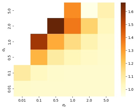
fig 4. overpaying ratio improvement depending on market
The values on the heatmap are given by: \(\frac{\text{overpayment ratio w/o feature}}{\text{overpayment ratio with feature}}\).
Higher values represent higher reduction in overpayment.
One can observe that as we incorporate more informative features (with a higher \(\sigma_x\)), the reduction in overpaying becomes more pronounced.
Takeaway
- Simply reducing your bids is not an efficient strategy to decrease overpayment in your production system.
- Incorporating informative features into your win probability model can significantly reduce overpaying.
- The market landscape also impacts overpayment metrics; inherently volatile markets may naturally exhibit high overpayment metric values.
References
- Log-normal distribution